Easy-to-Understand Food Microbiology Testing Sampling Plans in the ICMSF

The meaning of a "negative" result in food microbiological testing varies depending on the sampling plan used. This article aims to explain the sampling plans of the International Commission on Microbiological Specifications for Foods (ICMSF) in an accessible manner. These sampling plans are adopted in the EU's food safety and process hygiene standards. Understanding the rationale behind these sampling plans is more important than memorising the plans themselves. This article focuses on explaining the "why" for beginners.

The Meaning of "Negative" in Food Microbiological Testing

When a negative result for Salmonella is reported for a batch of food, it’s important to consider what "negative" actually means.

Was only one sample tested and found negative?
Were five samples tested and all negative?
Were 30 samples tested and all negative?

A man and a woman looking puzzled at a laptop, with thought bubbles reading “They say Salmonella negative” and “What kind of sampling plan it was?”, highlighting the importance of understanding the sampling plan behind microbiological test results.

The interpretation of a negative result depends on the sampling plan used.

Illustration comparing two sampling approaches where inspectors report “Negative!”, while undetected contamination remains in a pallet, emphasising that a negative result depends on the sampling method.

This article discusses the sampling plans adopted in the EU’s food safety and process hygiene standards. These plans are essentially based on those set by the International Commission on Microbiological Specifications for Foods (ICMSF).

For beginners in food microbiology, this article will first explain the key points essential to understanding these sampling plans.

Types of ICMSF Sampling Plans and Their Purposes

ICMSF sampling plans can be broadly classified as follows:

Two-class plan (Class 2): Primarily qualitative
Three-class plan (Class 3): Quantitative

Note: Although some quantitative sampling plans are classified under the two-class plan, it is easier to understand the two-class plan as qualitative for now.

The microorganisms targeted in sampling tests are categorised as follows:

Pathogenic bacteria like Salmonella (high risk)
Indicator bacteria like E. coli (low risk)

Microbiological standards in the EU are broadly divided into:

Food Safety Criteria: Non-compliance requires product recall
Process Hygiene Criteria: Non-compliance requires a review of process control measures

For more detail, see the related article: “Differences in Microbiological Standards for Food in Japan and the EU, and Reasons for the Abolition of Hygiene Standards for Bento and Prepared Foods with HACCP Implementation.”

The relationship between sampling plans and these criteria can be summarised in the following table:

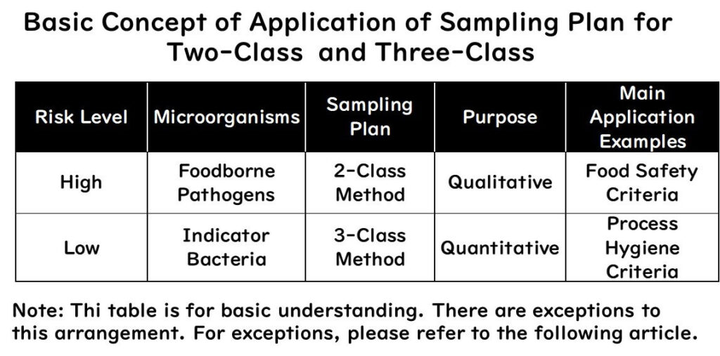
Table summarising the basic application of two-class and three-class sampling plans: high-risk foodborne pathogens use qualitative two-class methods for food safety criteria, while low-risk indicator bacteria use quantitative three-class methods for process hygiene criteria.

Reasons for the Above Summary

High-risk pathogens like Salmonella must not be present in food. Therefore, qualitative assessment (positive or negative) is used, leading to a two-class sampling plan. This is primarily used in food safety criteria in the EU.
Low-risk indicator bacteria are assessed quantitatively, meaning they must not exceed a certain amount. This leads to a three-class sampling plan, mainly used in process hygiene criteria in the EU.

Two-Class Sampling Plan (Qualitative)

A two-class sampling plan is a qualitative method that provides a binary result (presence or absence). This method is essential for pathogens that must not be present in food, such as foodborne illness-causing bacteria. Think of it as a red-card situation: a binary decision.

Cartoon-style image illustrating a two-class qualitative sampling plan, with a referee character showing a red card to a blue microbe, symbolising zero tolerance for pathogens—“one shot away” from rejection.

The diagram below shows the sampling plan for Salmonella in the EU’s food safety criteria for various products such as minced meat, raw poultry, egg products, cooked shellfish, and ice cream:

n: Number of samples
m: Safety standard value
c: Acceptable number of positives

The following applies:

Five samples must be tested (n = 5)
No detection in 25g of the sample (m = 0/25g)
Not a single sample exceeding the standard is acceptable (c = 0)

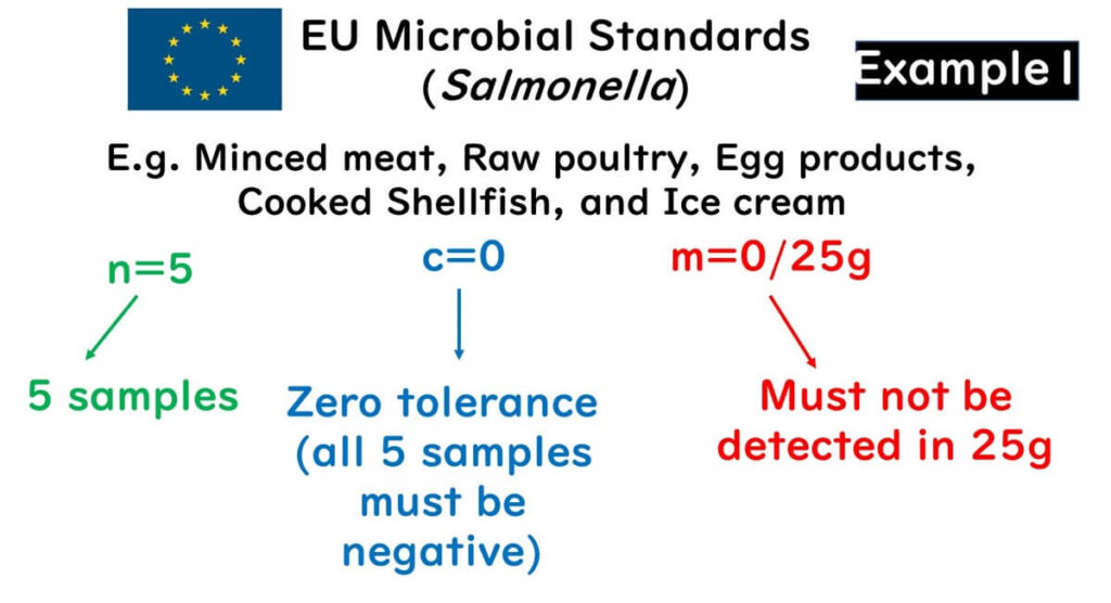
Diagram explaining EU microbial standards for Salmonella in foods like minced meat and egg products, showing a two-class plan with five samples (n=5), zero tolerance (c=0), and non-detection required in 25g (m=0/25g).

Most of the EU's food safety standards for Salmonella are set at n = 5.

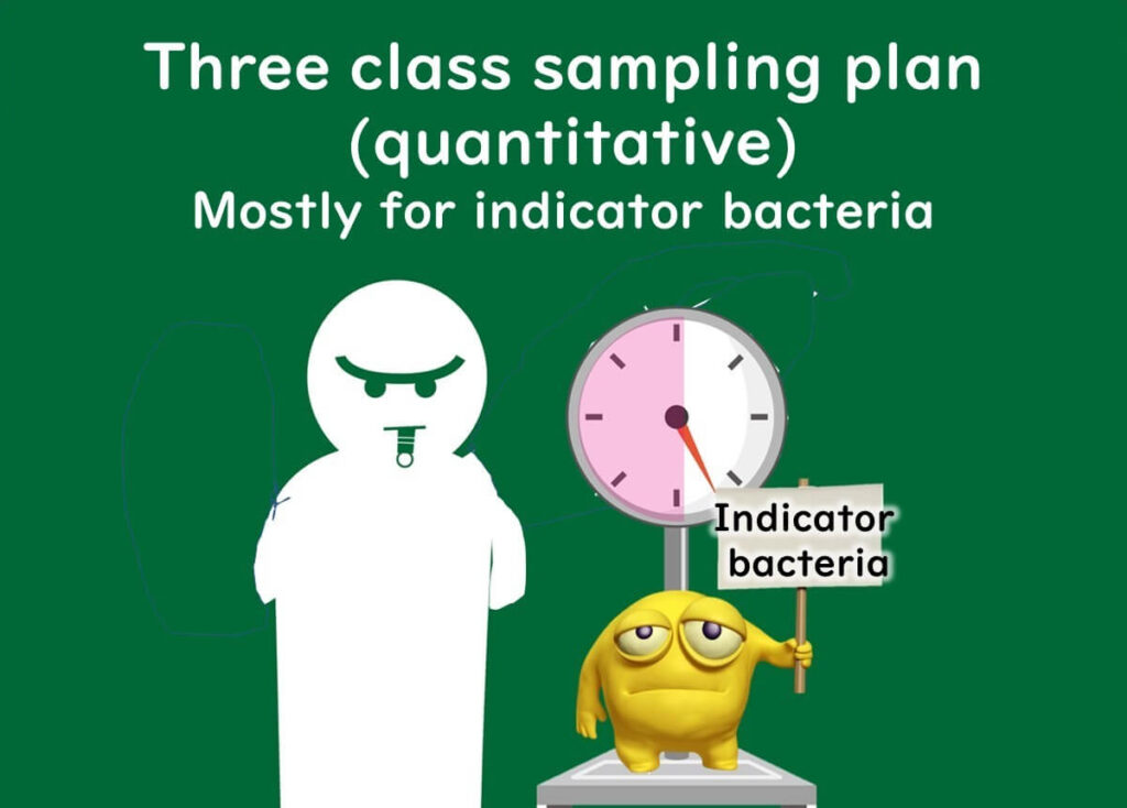
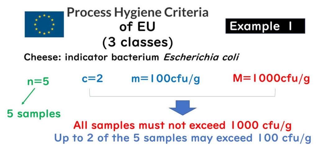
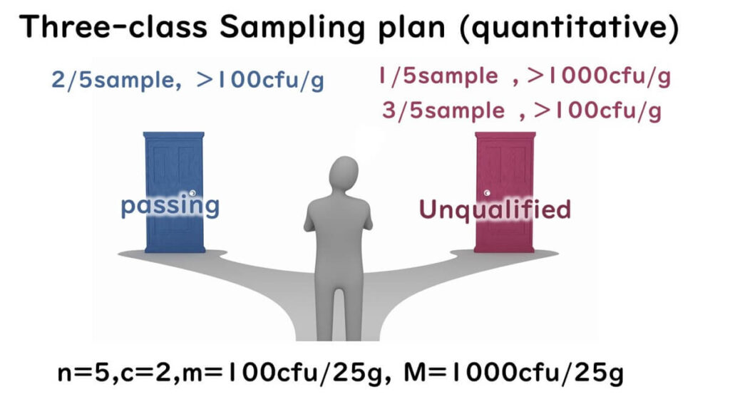
Three-Class Sampling Plan (Quantitative)

While the two-class sampling plan involves a qualitative decision, the three-class sampling plan incorporates quantitative elements.

In the EU, this plan is used for indicator bacteria rather than pathogens and is applied in process hygiene criteria rather than food safety criteria.

Note: Exceptions exist.

Cartoon illustration of a three-class quantitative sampling plan used mainly for indicator bacteria, featuring a judge-like character, a gauge, and a yellow microbe holding a sign reading “Indicator bacteria”.

The diagram below shows the sampling plan for E. coli as an indicator bacterium in a cheese manufacturing plant under the EU’s process hygiene criteria. The plan is defined by (n, c, m, M).

For example:

n = 5: Five samples need to be tested
m = 100 cfu/g, c = 2: Up to two of the five samples can exceed 100 cfu/g
M = 1000 cfu/g: If even one sample exceeds 1000 cfu/g, it is non-compliant

Diagram illustrating EU process hygiene criteria for cheese using a three-class sampling plan for Escherichia coli: five samples (n=5), with up to two allowed to exceed 100 cfu/g (c=2, m=100 cfu/g), but none may exceed 1000 cfu/g (M=1000 cfu/g).

The diagram illustrates scenarios of pass and fail outcomes:

Up to two out of five samples exceed 100 cfu/g, none over 1000 cfu/g → Pass
One sample exceeds both 100 cfu/g and 1000 cfu/g → Fail
Three samples exceed 100 cfu/g, regardless of 1000 cfu/g → Fail

Illustration of a decision point in a three-class quantitative sampling plan, showing criteria for passing (e.g. 2 out of 5 samples exceed 100 cfu/g) versus failing (e.g. 1 sample exceeds 1000 cfu/g or 3 exceed 100 cfu/g), based on n=5, c=2, m=100 cfu/25g, M=1000 cfu/25g.

Sampling Plan Design Strategy

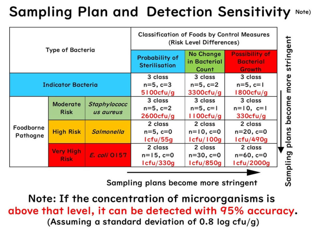
The table below provides general guidelines for which sampling plan to use based on microorganisms and food types.

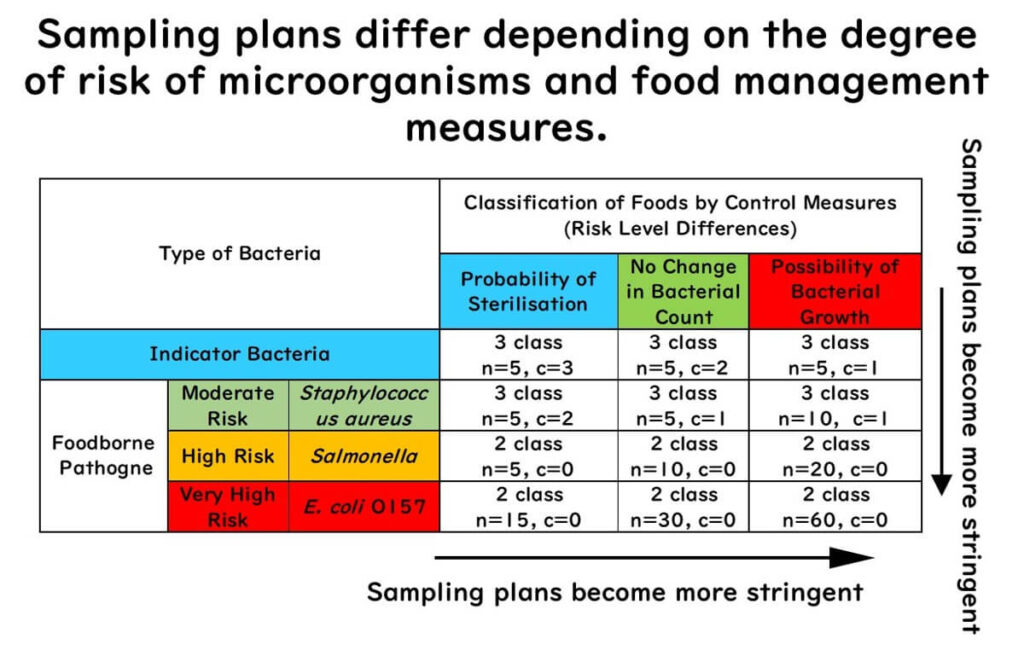
Matrix showing how microbiological sampling plans vary by bacterial risk level and food management conditions, with stricter criteria applied to higher-risk pathogens and foods where bacterial growth is likely; includes examples like Staphylococcus aureus, Salmonella, and E. coli O157 under different sampling plans.

The stringency (detection sensitivity) of a sampling plan is determined by several factors:

Two-class plans are stricter than three-class plans, with no tolerance for deviation
In any plan, increasing n and decreasing acceptable positives (c) increases stringency
Microorganisms vary in risk:
- Low (indicator bacteria)
- Moderate (e.g. Staphylococcus aureus)
- High (e.g. Salmonella)
- Very high (e.g. E. coli O157)
Food management depends on whether food can be sterilised and whether bacteria may multiply during distribution

Strategy Summary

As microorganism risk increases, the sampling plan becomes stricter
Foods that can be sterilised may have more lenient plans; if bacterial growth is possible during distribution, stricter plans are needed

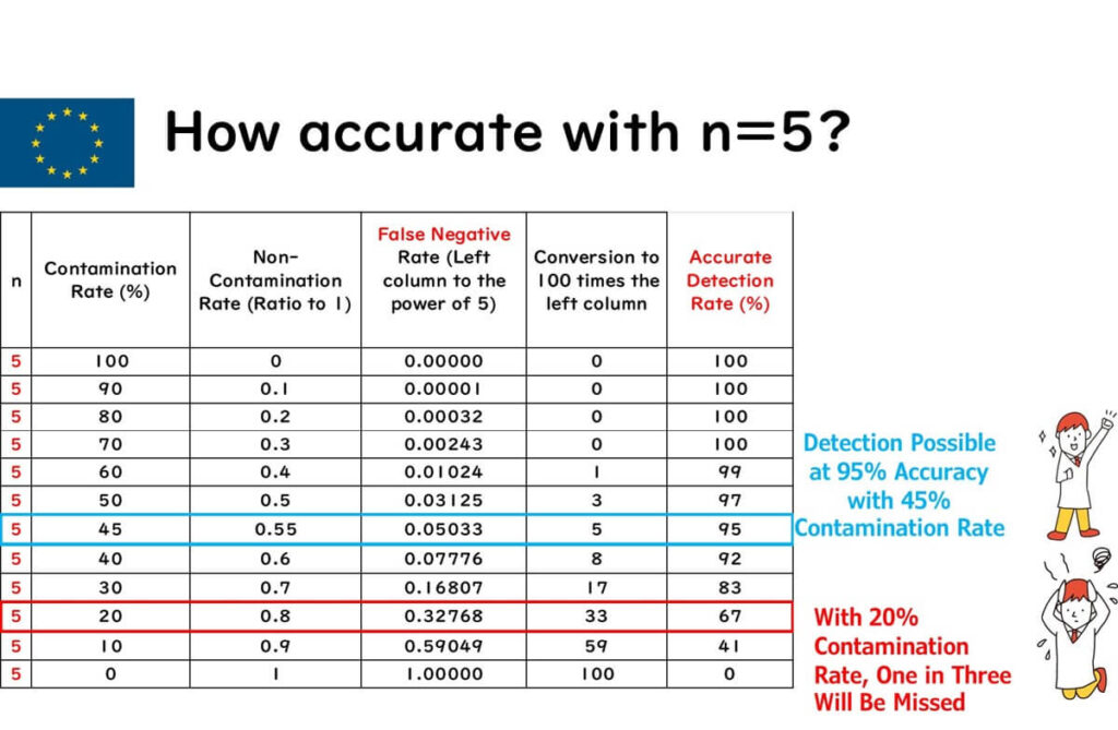
Accuracy of Sampling Plans

How accurate are these sampling plans?

Example 1: Salmonella Sampling Plan with n = 5 in the EU

The chart below shows the probability of detecting various Salmonella contamination rates when testing five samples.

Table showing detection accuracy for n=5 sampling in relation to contamination rates. At 45% contamination, detection accuracy is 95%, while at 20% contamination, one in three cases may be missed. Includes false negative rates, conversion values, and highlights of key thresholds.

For beginners, a separate article includes a step-by-step explanation and video guide on the creation of this table and calculation of testing accuracy.

From the chart:

At a 45% contamination rate, detection probability is 95%
At a 20% contamination rate, detection drops to 67% — one in three tests could miss it (false negative)

Example 2: Salmonella Sampling Plan with n = 30 for Infant Formula

For infant formula in the EU:

n = 30
No detection in 25g (m = 0/25g)
No positives allowed (c = 0)

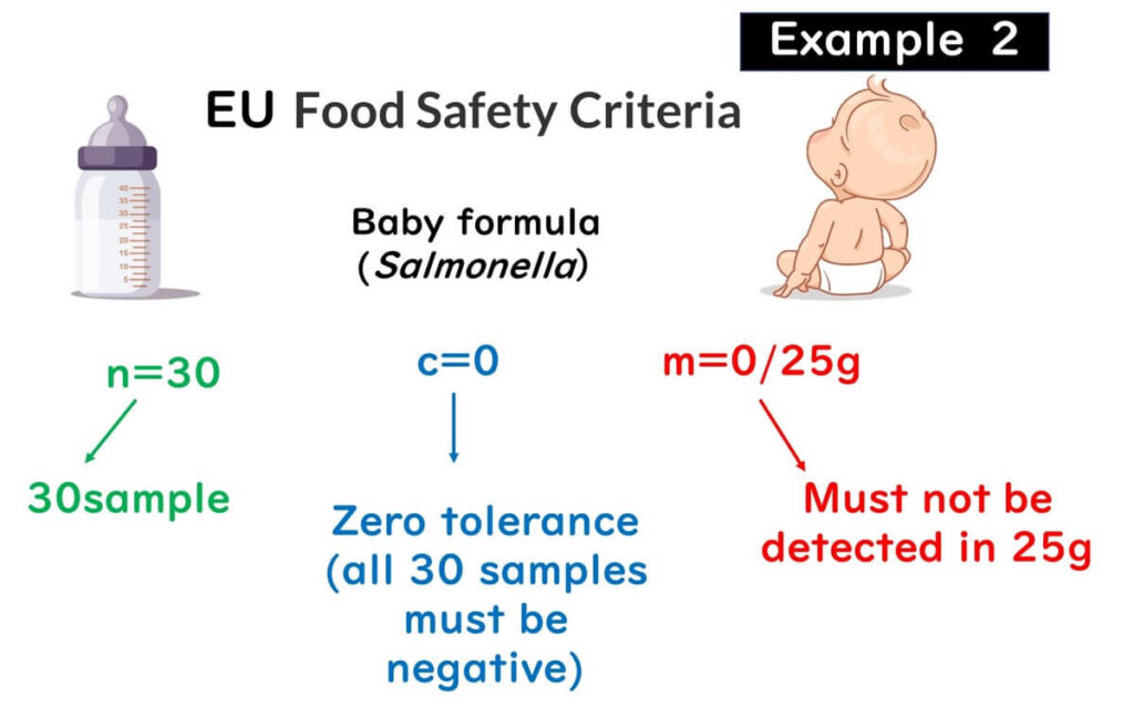
Illustration of EU food safety criteria for baby formula regarding Salmonella, showing a two-class sampling plan requiring 30 samples (n=30), with zero tolerance (c=0) and no detection permitted in 25g of any sample (m=0/25g).

The ICMSF recommends n = 60, but EU uses n = 30.

The chart below shows detection probability for different contamination rates with n = 30.

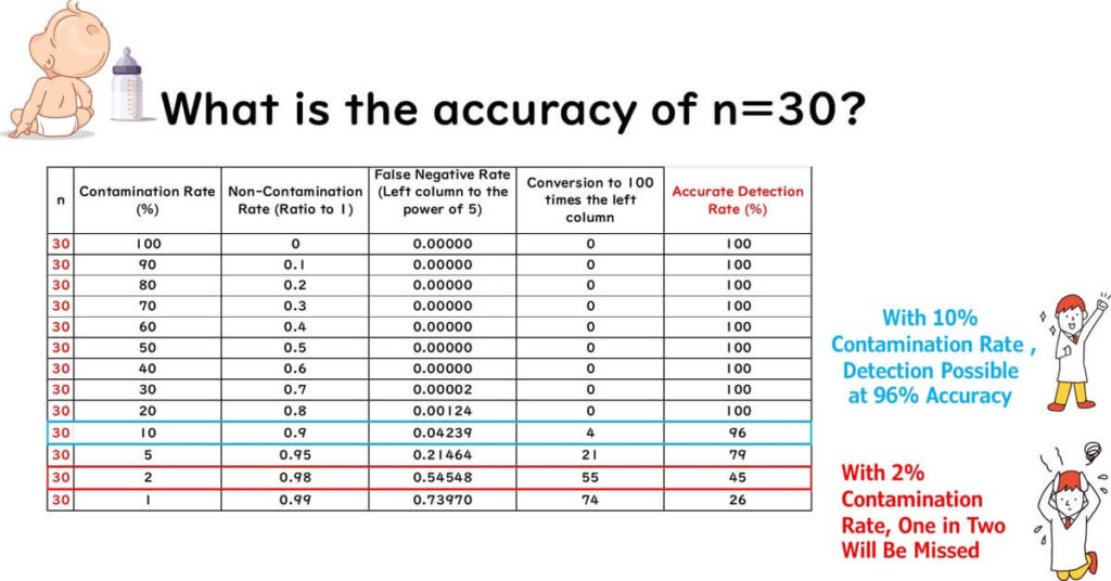
Table showing detection accuracy for n=30 samples at varying contamination rates. At 10% contamination, accuracy is 96%, while at 2% it drops to 45%, meaning half of cases may be missed. Includes false negative rates and illustrated messages emphasising detection challenges at low contamination levels.

From the chart:

At 10% contamination rate, detection probability is 96%
At 2% contamination rate, detection probability drops to 45% (1 in 2 false negative)

Relationship Between Sampling Plans and Food Safety Evaluation

As discussed, increasing the sample number n cannot eliminate all risk. Without testing every unit, 100% certainty is unachievable.

So, are these sampling plans still meaningful?

Surprised man pointing at a leaking pipe labelled “Microbiology Tests”, with a speech bubble asking “Is this test trustworthy?”, symbolising doubts about the reliability of microbiological testing methods.

Yes.

A properly designed sampling plan allows reasonable estimation of microbial concentration (microbial load)

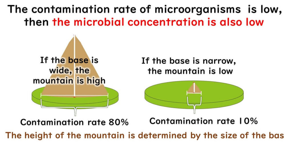
Lower Contamination Rates Indicate Lower Microbial Load

There is a correlation between contamination rate and microbial load:

Lower contamination rate → lower average microbial concentration

Think of it as a mountain: a narrow base suggests a small hill; a wide base may mean a towering peak like Mount Fuji.

Diagram comparing microbial contamination rates using mountain analogies: a wide base with 80% contamination represents high microbial concentration, while a narrow base with 10% contamination indicates low concentration. Emphasises that microbial load is related to the contamination rate.

To explain further, consider Russian Roulette:

One bullet (10%) or ten bullets (100%) — either way, pulling the trigger can be fatal

Image of a concerned man pointing towards a revolver with one bullet loaded, illustrating the concept of Russian Roulette, accompanied by the message “One bullet can be fatal” to highlight high-risk scenarios such as severe microbial contamination.

But microbiological testing isn’t Russian Roulette.

Image contrasting microbiological testing with Russian Roulette, showing a relieved man and a crossed-out revolver, accompanied by the message “Don’t think in Russian roulette”, to emphasise that food testing should not be viewed as a fatal-risk gamble.

In food testing, fewer "bullets" (lower contamination rate) mean even if hit (positive result), the impact (concentration) may be minimal.

Cartoon-style image showing a man shrugging while a revolver fires a slow-moving bullet, with a speech bubble saying “The bullet is slow, so it's no big deal,” metaphorically downplaying risk—used to contrast slow microbial contamination with the perception of danger.

Why?

Microorganism distribution in food often follows a log-normal distribution:

When graphed on a logarithmic scale, the curve is symmetrical
The highest probability lies at the mean
Probability decreases as values diverge from the mean

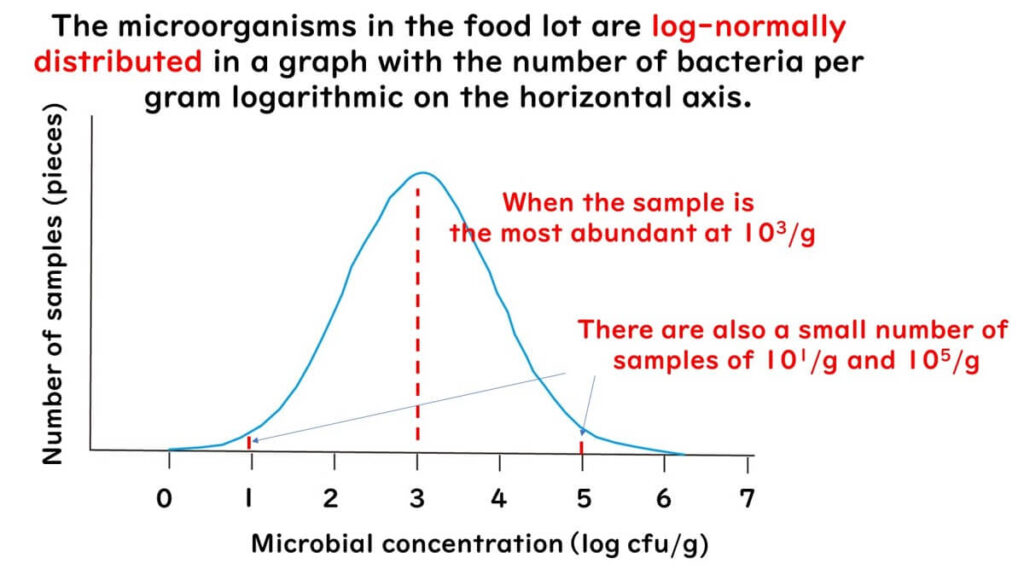
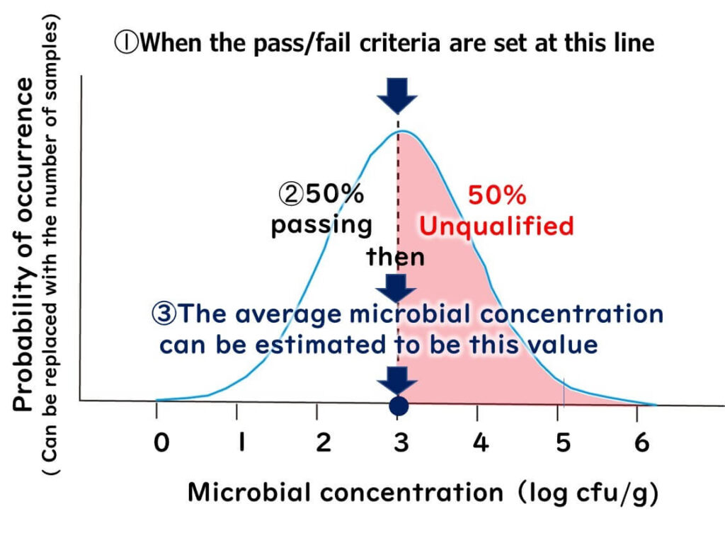
Graph showing a log-normal distribution of microbial concentrations in food samples, with the peak at 10³ cfu/g, and smaller numbers of samples at both low (10¹) and high (10⁵) concentrations, illustrating variability in microbial load across a batch.

For example, with a criterion of 10³/g:

If 50% of samples pass, the mean is 10³/g

Bell-shaped graph showing a log-normal distribution of microbial concentration, with pass/fail criteria set at log 3 (10³ cfu/g), where 50% of samples pass and 50% fail. The mean microbial concentration is estimated at the pass/fail threshold, illustrating how positive rates can indicate average contamination levels.

If 20% fail and 80% pass:

The mean shifts left to ~1.7 log = ~5×10¹/g

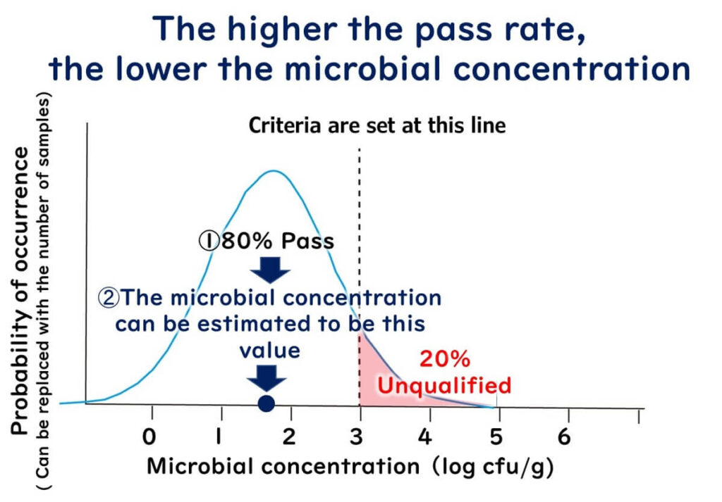
Graph illustrating that a higher pass rate (e.g. 80%) indicates a lower average microbial concentration. With the pass/fail criterion set at log 3 (10³ cfu/g), only 20% of samples are unqualified, and the estimated average microbial level is around log 2 (10² cfu/g).

Conclusion from the Above:

Lower contamination rate → lower average microbial concentration
Higher contamination rate → higher average microbial concentration

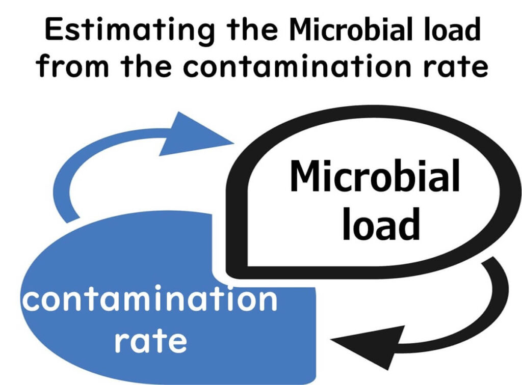
Estimating Contamination Levels from Contamination Rates

By applying the above principles, one can estimate microbial concentrations based on contamination rates.

Conceptual diagram illustrating the relationship between contamination rate and microbial load, with arrows indicating a cycle where contamination rate can be used to estimate microbial load.

However, estimation depends on the standard deviation, which defines the shape of the distribution.

Bell curve illustrating the importance of standard deviation in microbial distribution surveys, with a double-headed arrow showing how standard deviation defines the width of the distribution.

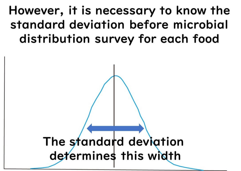
Standard deviation must be measured for each food type — it varies by food, microorganism, and process.

Once standard deviation is known, contamination rate from sample results can predict average microbial concentration for the batch.

If no prior data exists, a default standard deviation value can be used.

This chart shows how a 30%, 50%, or 70% positive rate converts into average microbial concentrations (assuming a criterion of 10³ log cfu/g):

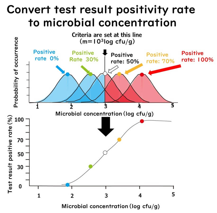
Diagram showing how different microbial concentration distributions (log cfu/g) correspond to varying test positivity rates, ranging from 0% to 100%. The lower graph illustrates a sigmoid curve converting positivity rate into estimated microbial concentration, with a criterion set at 10³ cfu/g.

30% positive → ~10².⁷ log cfu/g
50% positive → ~10³.⁰ log cfu/g
70% positive → ~10³.⁵ log cfu/g

Using this, the ICMSF provides expected microbial concentrations for various sampling plans at 95% detection probability:

Table comparing sampling plans and detection sensitivity by bacterial type and food control measures. Stricter plans apply to higher-risk pathogens and conditions favouring bacterial growth. Detection limits (e.g. 1 cfu/2000g for E. coli O157) correspond to 95% detection accuracy assuming a standard deviation of 0.8 log cfu/g.

This article does not cover the exact formulas. Understanding the concept is sufficient for most food microbiology practitioners.

Summary for Beginners

To summarise:

Even with a large number of samples, some contamination may be missed
However, based on sampling plan accuracy, one can estimate microbial concentrations at a 95% detection level
By selecting appropriate sampling plans tailored to the microorganism and food type, food safety risks can be effectively managed

Once these points are grasped, beginners will have a strong foundation.

Additional Information on ICMSF Sampling Plans

This section is for readers who understand the basics covered earlier.

ICMSF sampling plans include more than just the two described previously.

Illustration of a skier in motion under the heading “Further understanding of intermediate,” symbolising the progression from basic to intermediate-level knowledge, likely in the context of food microbiology or sampling plans.

Quantitative Two-Class Sampling Plan

Although two-class plans are often qualitative, ICMSF also defines quantitative two-class plans.

Example: EU standards for Listeria in ready-to-eat foods (where Listeria cannot grow during distribution):

Up to 100 cfu/g is allowed

Foods where Listeria can grow are held to zero tolerance (non-detectable in 25g)

For Listeria in non-growth environments:

n = 5, m = 100 cfu/g, c = 0

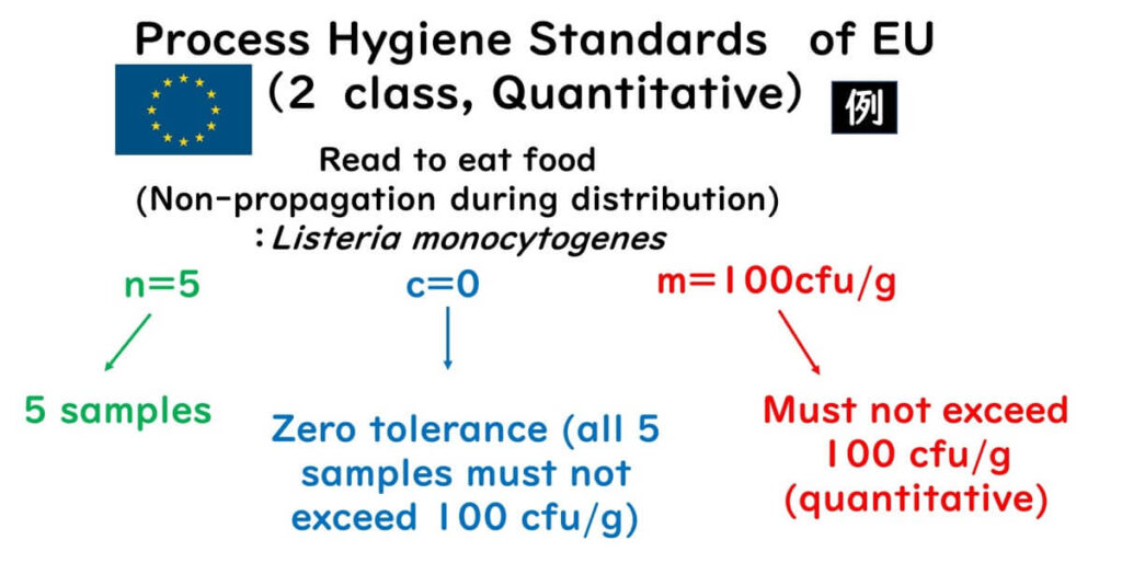
Diagram explaining the EU process hygiene standards for ready-to-eat foods where Listeria monocytogenes does not grow during distribution. A two-class quantitative plan requires five samples (n=5), with zero tolerance (c=0), and microbial counts not exceeding 100 cfu/g (m=100 cfu/g).

Comparison:

Qualitative: non-detectable in 25g
Quantitative: limit of 100 cfu/g

Hence, this is termed a quantitative two-class sampling plan.

"Qualitative + Quantitative" Mixed Sampling Plan

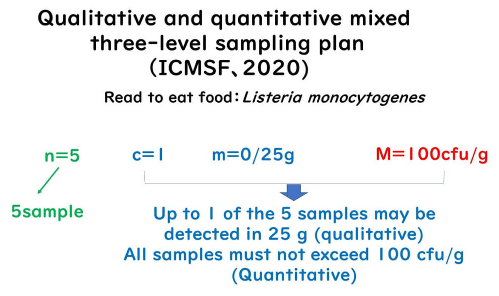
The mixed three-class sampling plan combines both approaches. Proposed by ICMSF in 2020 for Listeria in ready-to-eat foods.

For details, see Marcel H. Zwietering’s ICMSF 2020 video presentation.

Summary:

n = 5
m = 0/25g (Listeria must not be detected)
c = 1 (1 sample exceeding allowed)
M = 100 cfu/g: if any sample exceeds this, it fails

Illustration of the ICMSF (2020) mixed three-level sampling plan for Listeria monocytogenes in ready-to-eat foods. The plan allows one positive out of five samples (n=5, c=1) in 25g (qualitative), but none may exceed 100 cfu/g (M=100 cfu/g, quantitative).

Why Introduce This Plan?

Reference: Farber et al., Food Control, May 2021

The zero-tolerance two-class plan has drawbacks:

Frequent recalls and economic losses
Manufacturers may avoid voluntary testing due to fear of recalls

The mixed plan allows flexibility while maintaining safety:

Detection sensitivity remains high, often stricter than zero-tolerance plans in the US (n = 1 or 2)

Conclusion

Sampling plans in food microbiology are essential. Understanding the basic principles, especially the rationale behind them, is critical for beginners.

However, detailed calculations are not required for most practitioners. Understanding the direction and purpose of sampling plans is sufficient; technical computations can be left to experts.

Cartoon of a woman speaking to a statistician in front of a whiteboard filled with complex equations. She says, “I’ll leave the detailed calculations to you,” while the caption below reads, “I’ve been re-calculating my career,” humourously illustrating the intimidating nature of statistical analysis.

For more information on ICMSF sampling plans, visit the ICMSF website, which offers books and educational videos.

Categories: Microbial Testing in HACCP

The Meaning of "Negative" in Food Microbiological Testing